Phylogeny Construction with SNPs

Better explanaitions in our wiki: Wiki

Or the R Markdown with all the commands >file<

Or a full population genetics R pipeline in GrunLab

Pipeline

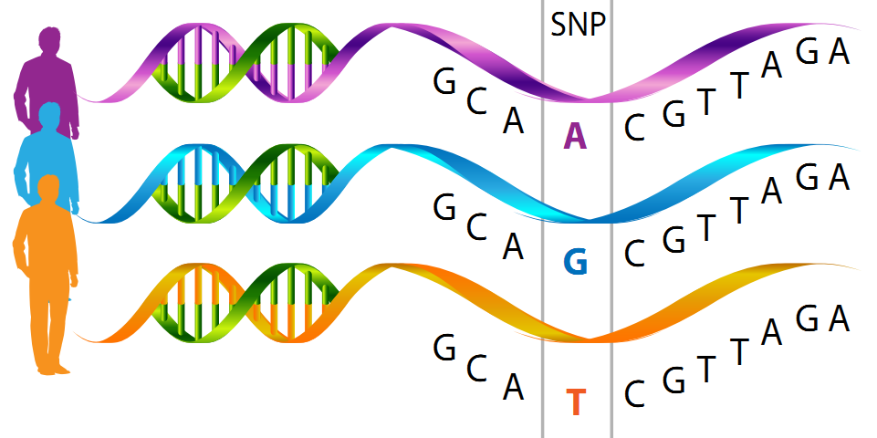
We received a vcf file where SNPsaurus converted genomic DNA into nextRAD genotyping-by-sequencing libraries (SNPsaurus, LLC). The nextRAD libraries were sequenced on a HiSeq 4000 on two lanes of 150bp reads.

With this pipeline you would be able to:

Modified from population genetics http://grunwaldlab.github.io/Population_Genetics_in_R/qc.html

Using RStudio 3.4.4 and packages:

genepop, parallel, poppr, dartR, devtools, phytools, seqinr, phylotools, adegenet, pegas, hierfstat

library(vcfR)
library(ggplot2)
library(reshape2)
install_github("whitlock/OutFLANK")
biocLite("qvalue")

library("genepopedit")
library("devtools")
library("pcadapt")
library("qvalue")
library("OutFLANK")
library("ggplot2")
library(genepop)
library(vcfR)
library(ade4)
...

Remove indels (insertions-deletions)

Muricea.vcf_ID_SNPs <- extract.indels(Muricea.vcf_ID,return.indels = FALSE)
Muricea.vcf_ID_SNPs  
Muricea.vcf_ID_Indels <- extract.indels(Muricea.vcf_ID,return.indels = TRUE)
Muricea.vcf_ID_Indels

SNPs upper and lower 20% of depth distribution

   Muricea_dp<- extract.gt(Muricea.vcf_ID_SNPs, element = "DP", as.numeric=TRUE)

Delete:

3.1 Samples (missingness >70%)

Muricea.vcf_ID_SNPs_miss <- apply(Muricea.vcf_ID_SNPs_dp, MARGIN = 2, function(x){ sum(is.na(x)) })
Muricea.vcf_ID_SNPs_miss <- Muricea.vcf_ID_SNPs_miss/nrow(Muricea.vcf_ID_SNPs_dp)*100

3.2 SNPs - variants (>90%) with high degree of missingness information

Muricea_miss <- apply(Muricea_dp, MARGIN = 1, function(x){ sum( is.na(x) ) } )
Muricea_miss <- Muricea_miss / ncol(Muricea_dp)*100
Muricea_DP_filtered <- Muricea.vcf_ID_SNPs[Muricea_miss<90]

Rewrite vcf file

   write.vcf(Muricea_DP_filtered,file= "Muricea_DP_90Miss_filtered.vcf")

Using RStudio or VCFTOOLS 0.1.17

Run Minor Allele Frequency (MAF)

 Muricea_MAF_vcf <-maf(Muricea_DP_90Miss_filtered.vcf)
 Muricea_MAF_vcf[Muricea_MAF_vcf[,4]< 0.01]<- NA 
 Muricea_MAF_vcf_NA <- is.na(Muricea_MAF_vcf[,4])
 Muricea_MAF_vcf_NA_loci<- which(Muricea_MAF_vcf_NA, arr.ind = TRUE, useNames = TRUE)
   
 Muricea_toRemoveMAF<- c(Muricea_MAF_vcf_NA_loci)
 length(Muricea_toRemoveMAF)
 Muricea_filtered_no_clone_DP_Miss90_MAF_vcf_last <- Muricea_DP_90Miss_filtered.vcf[-Muricea_toRemoveMAF]

Convert VCF file to genind and distance matrix

genind_Muricea <- vcfR2genind(Muricea_filtered_no_clone_DP_Miss90_MAF_vcf_last)
genind_Muricea
Muricea_distances_FINAL.dist<-diss.dist(genind_Muricea, mat=TRUE, percent = TRUE)

write.table(Muricea_distances_FINAL.dist, file="Muricea_distances_FINAL.dist.txt", col.names = TRUE, row.names = TRUE, quote = FALSE)

write.csv(Muricea_distances_FINAL.dist, file="Muricea_distances.dist_FINAL.csv", col.names = TRUE, row.names = TRUE, quote = FALSE)

Generate visualization plots

To verify quality filters

Heatmaps

  heatmap.bp(Muricea_DP_70Miss_MAF01_Bialle_LD150_filtered.vcf_dp[1:1000,], rlabels = FALSE)

Barplots
Violinplots

  dp <- extract.gt(Muricea_DP_90Miss_filtered.vcf,  element = "DP", as.numeric = TRUE)
  class(dp)


  dpf <- melt(dp, varnames = c("Index", "Sample"),
              value.name = "Depth", na.rm = TRUE)
  dpf <- dpf[ dpf$Depth > 0, ]
  p <- ggplot(dpf, aes(x = Sample, y = Depth))
  p <- p + geom_violin(fill = "#C0C0C0", adjust = 1.0,
                       scale = "count", trim = TRUE)
  p <- p + theme_bw()
  p <- p + theme(axis.title.x = element_blank(),
                 axis.text.x = element_text(angle = 60, hjust = 1))
  p <- p + scale_y_continuous(trans = scales::log2_trans(),
                              breaks = c(1, 10, 100, 800),
                              minor_breaks = c(1:10, 2:10 * 10, 2:8 * 100))
  p <- p + theme(panel.grid.major.y = element_line(color = "#A9A9A9", size = 0.6))
  p <- p + theme(panel.grid.minor.y = element_line(color = "#C0C0C0", size = 0.2))
  p <- p + ylab("Depth (DP)")
  p

Convert vcf file to PHYLIP format

Suitable for RAxML

Or you can use another tool from CIPRESS Phylogenetic Collection (BEAST2, MRBAYES, RAXML) CyVerse

Need:

References

GrunLab
RStudio: A Platform‐Independent IDE for R and Sweave - Racine - 2012 - Journal of Applied Econometrics - Wiley Online Library. https://onlinelibrary.wiley.com/doi/abs/10.1002/jae.1278.
variant call format and VCFtools Bioinformatics Oxford Academic. https://academic.oup.com/bioinformatics/article/27/15/2156/402296.
Lischer, H. E. L. & Excoffier, L. PGDSpider: an automated data conversion tool for connecting population genetics and genomics programs. Bioinformatics 28, 298–299 (2012).
Stamatakis, A. RAxML version 8: a tool for phylogenetic analysis and post-analysis of large phylogenies. Bioinformatics 30, 1312–1313 (2014).
Miller, M. A., Pfeiffer, W. & Schwartz, T. The CIPRES Science Gateway: Enabling High-impact Science for Phylogenetics Researchers with Limited Resources. in Proceedings of the 1st Conference of the Extreme Science and Engineering Discovery Environment: Bridging from the eXtreme to the Campus and Beyond 39:1–39:8 (ACM, 2012). doi:10.1145/2335755.2335836.
Letunic, I. & Bork, P. Interactive Tree Of Life (iTOL) v4: recent updates and new developments. Nucleic Acids Res. 47, W256–W259 (2019).
https://www.onworks.net/programs/vcftools-online?amp=0

___________________

Future pipeline:

Learn the SNPs format
SNPs calling
SNPs filtering 3.1. Samples quality 3.2. Variants quality